The Science Behind QPlants

How QPlants Works

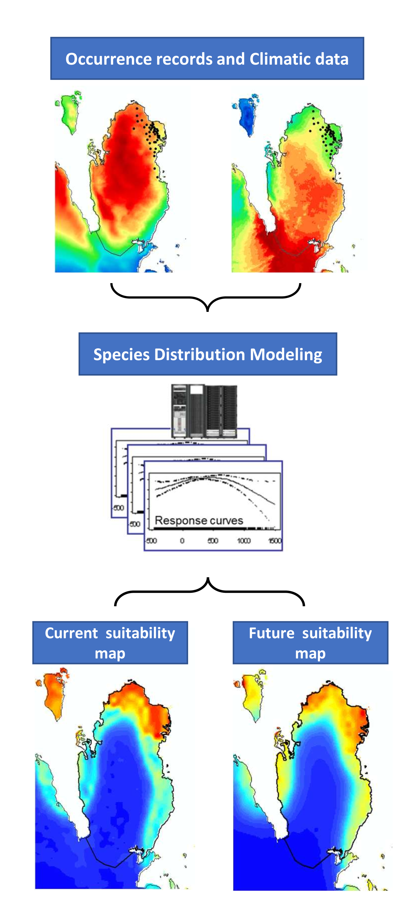
From plant records to future climate predictions

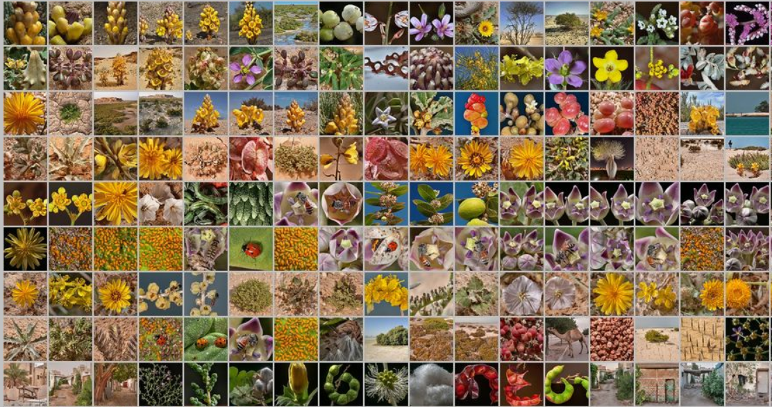
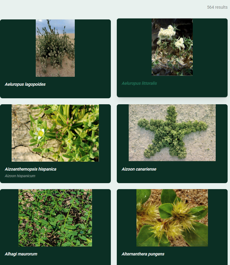
Qatar Plant Database (QPlants) is the first comprehensive digital platform dedicated to Qatar's flora, bringing together information for more than 550 plant species across the country.

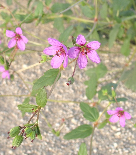
Erodium glaucophyllum — one of Qatar's documented species

Why This Matters

Understanding how climate affects plant distributions is essential for protecting Qatar's biodiversity in a rapidly changing environment. As temperatures rise and environmental conditions shift, some species may lose suitable habitats while others may expand into new areas.

QPlants helps identify vulnerable species, future climate refuges, and regions that may remain suitable for plant survival under future climate scenarios. These insights can support biodiversity conservation, ecological restoration, sustainable land management, and future environmental planning across Qatar.

Conservation

Identify vulnerable species and future climate refuges to prioritise protection efforts.

Research

Provide researchers and decision-makers with scientifically grounded data on climate impacts.

Planning

Support land management, restoration planning, and ecological resilience strategies.

How We Predict Plant Habitats

One of the main goals of QPlants is to show where different plant species can grow now and how their suitable habitats may change in the future. To do this, we created maps that estimate how suitable the climate is for each species across different regions.

These maps are based mainly on climate conditions such as temperature and rainfall. By combining climate data with information about where plants have already been found in nature, we can estimate where conditions are favorable for each species today and where they may become favorable or unfavorable as the climate changes.

Understanding plant "climate suitability"

Every plant species can survive only within a certain range of environmental conditions. For example, some plants tolerate extreme heat and drought, while others require cooler temperatures or more rainfall. Scientists often refer to this set of suitable conditions as a species' "ecological niche" — the type of environment where a species can live and reproduce successfully.

At large geographic scales, climate is usually the most important factor determining where plants can grow. Therefore, by understanding the climate preferences of a species, we can estimate its potential distribution across a landscape. To generate these habitat maps, QPlants combines biodiversity records with high-resolution climate datasets.

Where plant data comes from

To understand where each species occurs naturally, we gathered records from major global biodiversity databases, including scientific collections and verified public observations. These databases contain information from herbaria, research projects, and citizen science initiatives worldwide.

Because many species found in Qatar also occur in other dry regions, we included records from a wide area covering arid and semi-arid parts of the Middle East, the Mediterranean region, and nearby parts of Asia. This helped ensure that we captured the full range of environmental conditions in which each species can survive.

Before using these records, we carefully cleaned the data. We removed inaccurate locations, duplicate records, and observations with uncertain identification. Only species with enough reliable records were included in the analysis to ensure meaningful results.

Climate data used in the analysis

We used high-resolution global climate datasets that describe temperature and rainfall patterns over several decades. These datasets represent average conditions for the recent past and are widely used in environmental research.

In addition to current climate conditions, we also used projections of future climate based on international climate models. These projections estimate how temperature and precipitation may change later in the century under different greenhouse-gas emission scenarios.

Because future climate predictions involve uncertainty, we used several models and scenarios and combined their results to produce more reliable estimates.

Building the habitat suitability maps

To estimate suitable habitats, we used computer models that learn the relationship between plant locations and environmental conditions. In simple terms, the models identify the types of climates where a species is known to occur and then search for other places with similar conditions.

To increase reliability, we used several modeling methods rather than relying on a single one. The results from these methods were combined to produce a final map for each species.

We also tested how well the models performed by checking how accurately they predicted known plant locations. Only well-performing models were used in the final results.

Current and future habitat suitability

First, we produced maps showing areas that are climatically suitable under present conditions. Then we projected the same models onto future climate scenarios to estimate how suitable areas may shift over time.

For each species, we produced maps representing:

Current climate suitability
Suitability in the late 21st century under moderate climate change
Suitability under more severe climate change

Current suitability

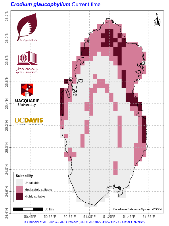
Erodium glaucophyllum current climate suitability map

2070 — SSP3 scenario

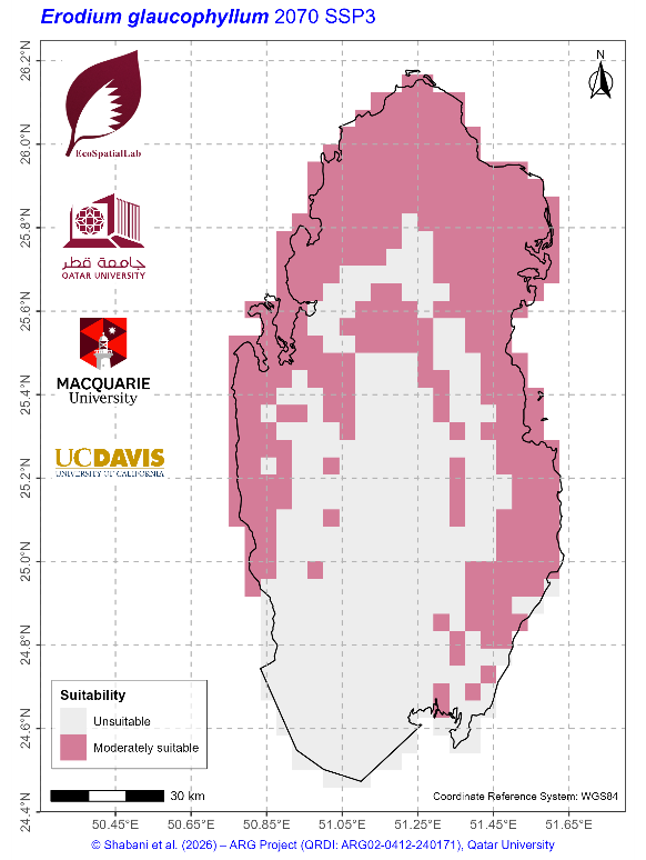
Erodium glaucophyllum projected suitability 2070 SSP3

Suitability values range from low to high, indicating how favorable the climate is for the species.

What these maps mean (and what they do not)

Climate suitability maps show where environmental conditions are likely to support a species. However, they do not guarantee that the species currently exists in those areas or that it will successfully establish there.

Other factors also influence plant distributions, including:

Soil type
Land use
Water availability
Competition with other species
Human activities

Therefore, the maps should be interpreted as indicators of potential suitability rather than exact predictions of presence.

Mapping habitat change (loss and gain)

To better understand potential changes, we compared current and future maps. This allowed us to estimate:

Areas that may become unsuitable for a species (habitat loss)
Areas that may become newly suitable (habitat gain)
Areas likely to remain suitable

These estimates help identify species that may be vulnerable to climate change as well as regions that could support them in the future.

Want to explore the science behind the models?

For researchers and users interested in the scientific methodology, the sections below describe the ecological concepts, climate datasets, and species distribution modeling approaches used to generate the habitat suitability maps.

Read the methodology ↓

Ecological Niche and Species Distribution Modeling (SDM)

Technical Methodology

In ecology, a niche is the match of a species to a specific environmental condition. It describes how an organism or population responds to the distribution of resources (Anderson et al., 2011). These resources can include a wide variety of abiotic (e.g., climate, soil, topography) and biotic (e.g., competitors, prey-predators, etc.) components. The type and number of variables comprising the dimensions of an ecological niche vary from one species to another and the relative importance of particular environmental variables for a species may vary according to the geographic and biotic contexts. But at large scales abiotic filters mostly affect ecological niche, among which, climatic variables are the most influential ones.

The geographic range, i.e., distribution of a species can be viewed as a spatial reflection of its ecological niche (Elith et al., 2010). In this regard, Species Distribution Modeling uses statistical models to predict the distribution of a species across geographic space and time using environmental data. The environmental variables are assumed to be factors that influence the distribution of the species. These variables are most often climate data (e.g., temperature, precipitation), but at local scales it can include variables such as soil type, topography, and land cover. When using climatic data, it is also possible to model species distribution for the current time and then projecting it to the future climatic conditions (for example 2050, 2070, or 2100). Methodologically speaking, SDM consists of three main components. The first part is occurrence records of the target species which can be compiled from online databases [for example Global Biodiversity Information Facility (GBIF) or iNaturalist] or collected during direct field surveys, or both. The second part is a set of predictors which comes from spatial raster maps. These raster maps are either already been created (such as climatic variables) or required to be preprocessed in GIS software. And the third part is a statistical model that uses values of the variables (raster maps) at occurrence points to fit a model and then predict the presence probability for all other places. In terms of climatic variables, it is possible to project the fitted model to other time periods, such as future scenarios.

Occurrence Records

For QPlants we used different sources to collect a sufficient and complete number of occurrence points for each plant species. We mainly downloaded occurrence points from GBIF and iNaturalist. These two databases contain details of plant specimens in herbaria, and observations from scientific and citizen science projects, from across the world. To ensure accessing a sufficient number of points for SDM analysis we defined a large spatial rectangle comprising all arid and semi-arid ecosystems of the Middle East, Mediterranean Basin, Central and Southern Asia. For each plant, we downloaded occurrence points inside this larger study area, merged them, and did some necessary preprocessing approaches to make them ready for the SDM analysis. We cleaned outlier points, removed those with no precise coordinates, double-checked their scientific names and combined those with synonymous names. We also removed duplicated points inside a 5-km buffer around them to cope with spatial auto-correlation. After all these filtering processes, we retained plants that had more than 30 occurrence points for the SDM analysis. In addition to occurrence points, SDM analysis requires absence or pseudo-absence (background) points for fitting the model. Background points are representatives of the environmental conditions accessible to each species and can be selected randomly across the entire study area. However, since all locations of a study area have not been equally surveyed to record species occurrence points, the collected records suffer imbalanced spatial biases towards easy-access areas. Hence, a more reasonable alternative is to select background points with the same spatial biases as the occurrence points have — the approach which is so called background-weighting (Phillips et al., 2009). To do so, for each plant species we first created a kernel density map from its occurrence records and then used the resulting map to select 10,000 background points with the same distribution probability.

Climatic Data

To generate plant habitat suitability maps we only focused on climatic variables because in the large extent of this project climate is the most important variable. Climate data were obtained from CHELSA (v 1.2, Karger et al., 2017), which contains high-resolution climatology data spanning the earth's land surface. We used climatic raster with a spatial resolution of 30 arc-seconds (approximately 1 km × 1 km at the equator). CHELSA climatic data include 19 raster maps for the current time representing temperature and precipitation averages and variations over 30 years (1981–2010). Due to inherent high-correlation between climatic variables, for each species we calculated Variance Inflation Factor (VIF) of all climatic variables and retained only those with lower multi-collinearity (VIF < 10). CHELSA database provides access to future climatology data for two time periods; 2041–2070 and 2071–2100. Future climatic data are provided based on five different Global Circulation Models (GCMs) and three climate change scenarios called Shared Socio-economic Pathways (SSPs). Different SSPs are utilised to quantitatively capture the connection between climate change scenarios and socio-economic growth trajectories (Riahi et al., 2017). Given the uncertainty in future climatic models, it is necessary to use multiple GCMs and SSPs scenarios. Therefore, we used all five GCMs (GFDL, IPSL, MPI-ESM, MRI-ESM, UKESM) provided in CHELSA under two frequently used SSPs (SSP3-7.0 and SSP5-8.5) for projecting current climatic suitability models to two future periods (hereafter 2070 and 2100).

Species Distribution Modeling

To predict suitable habitats for plant species, we implemented species distribution modeling in R using the biomod2 framework (Thuiller et al., 2009). This framework has the advantage of combining several methods for modeling and provides a more robust and reliable output by building an ensemble prediction. We focused on five of the most commonly used algorithms for species distribution modeling: generalized additive models (GAM), generalized linear models (GLM), generalized boosting models (GBM), maximum entropy (MaxEnt), and random forest (RF). This combination was chosen to balance models' overfitting and underfitting (Merow et al., 2014). For each species, we performed 10 iterations in each modeling approach based on a cross-validation approach. We then measured the performance of the models using two common metrics: AUC (area under the receiver operating characteristic curve) and TSS (true skill statistic). The final ensemble model was generated given the median of the TSS of the initial models. For species with limited occurrence records, the use of ensemble modeling, species-specific variable selection, and performance-based model inclusion helped reduce overfitting and improve prediction stability.

For each plant species, the fitted models based on the current baseline condition were then projected onto each of the future climate scenarios. We then averaged the output of five GCMs to create final future suitability models for two time periods (2070 and 2100) and under two climate change scenarios (SSP3-7.0 and SSP5-8.5). Final model output for each species consisted of one ensembled climatic suitability map for current time and five suitability maps (representing the five GCMs) for both 2070 and 2100 time-periods and under two climate change scenarios (SSP3-7.0 and SSP5-8.5). The climatic suitability maps had values ranging from 0 (least climatically suitable) to 1 (most climatically suitable). For each time period and under each SSP scenario we then calculated the median of five GCM projections. By doing so we obtained four final suitability maps: 2070 – SSP3, 2070 – SSP5, 2100 – SSP3, and 2100 – SSP5. We also classified continuous suitability maps to binary (0 and 1) maps by using TSS as the binarization metric. We then used the binary habitat suitability maps to quantify range loss and range gain in the habitat suitability of the species. The percentage of range loss and gain was determined based on the number of pixels currently unsuitable but predicted to become suitable in the future (habitat gain), and the number of pixels currently suitable but projected to become unsuitable (habitat loss).

References

Anderson, R. P., Martínez-Meyer, E., Nakamura, M., Araújo, M. B., Peterson, A. T., Soberón, J., & Pearson, R. G. (2011). Ecological niches and geographic distributions (MPB-49). Princeton University Press.
Elith, J., Kearney, M., & Phillips, S. (2010). The art of modelling range‐shifting species. Methods in ecology and evolution, 1(4), 330–342.
Merow, C., Smith, M. J., Edwards Jr, T. C., Guisan, A., McMahon, S. M., Normand, S., Thuiller, W., Wüest, R. O., Zimmermann, N. E., & Elith, J. (2014). What do we gain from simplicity versus complexity in species distribution models? Ecography, 37(12), 1267–1281.
Phillips, S. J., Dudík, M., Elith, J., Graham, C. H., Lehmann, A., Leathwick, J., & Ferrier, S. (2009). Sample selection bias and presence‐only distribution models: implications for background and pseudo‐absence data. Ecological applications, 19(1), 181–197.
Riahi, K., Van Vuuren, D. P., Kriegler, E., Edmonds, J., O'Neill, B. C., Fujimori, S., Bauer, N., Calvin, K., Dellink, R., & Fricko, O. (2017). The Shared Socioeconomic Pathways and their energy, land use, and greenhouse gas emissions implications: An overview. Global environmental change, 42, 153–168.
Thuiller, W., Lafourcade, B., Engler, R., & Araújo, M. B. (2009). BIOMOD–a platform for ensemble forecasting of species distributions. Ecography, 32(3), 369–373.